Excel Formulas: Cell Color Based IF Statements

In the world of data analysis, Excel is a powerful tool that offers a wide range of functions and formulas to manipulate and analyze data. One useful feature in Excel is the ability to create worksheets, which allow users to organize and present their dataset in a structured manner. With Excel, users can easily define a data_range and perform various operations on the cell values within that range. This makes it efficient and convenient for users to work with their datasets and extract meaningful insights.

One useful feature in Excel is the ability to create worksheets, which allow users to organize and present their dataset in a structured manner. With Excel, users can easily define a data_range and perform various operations on the cell values within that range. This makes it efficient and convenient for users to work with their datasets and extract meaningful insights. However, did you know that you can go beyond traditional criteria and leverage cell color as a criterion in your Excel formulas? With the new cell_color feature, you can now easily getcellcolor and countcellsbycolor in your spreadsheets.

This allows you to efficiently analyze and manipulate data based on the fill colors of cells. So, take advantage of this powerful functionality to enhance your Excel formulas. With the new cell_color feature, you can now easily getcellcolor and countcellsbycolor in your spreadsheets. This allows you to efficiently analyze and manipulate data based on the fill colors of cells. So, take advantage of this powerful functionality to enhance your Excel formulas. This opens up new possibilities for organizing, categorizing, and analyzing dataset based on visual cues. The color column allows for changes in color cells, enhancing the ability to identify and analyze data.

By understanding how to use cell color as a criterion in Excel formulas, you can unlock the potential for more efficient data analysis. With functions like getcellcolor and countcellsbycolor, you can easily analyze and manipulate data based on cell_color. This allows for a more precise and targeted analysis, saving time and effort. So, don’t overlook the importance of considering cell_color in your Excel formulas – it can greatly enhance your data analysis capabilities. With functions like getcellcolor and countcellsbycolor, you can easily analyze and manipulate data based on cell_color.

This allows for a more precise and targeted analysis, saving time and effort. So, don’t overlook the importance of considering cell_color in your Excel formulas – it can greatly enhance your data analysis capabilities. Imagine being able to automatically calculate values or perform actions based on specific colors assigned to cells. With the new “getcellcolor” function, you can easily retrieve the “cell_color” of any cell in your spreadsheet. This allows you to “countcellsbycolor” and perform various operations based on the “colour” of the cells. With the new “getcellcolor” function, you can easily retrieve the “cell_color” of any cell in your spreadsheet. This allows you to “countcellsbycolor” and perform various operations based on the “colour” of the cells.

In this tutorial, we will explore the benefits of using Excel formulas based on cell color (cell_color) and guide you through examples of how to implement them effectively. These formulas allow you to perform calculations or apply specific actions based on the color of a cell (colour). By referencing the desired cell (cell_ref), you can easily manipulate data or highlight specific values. For example, you can use a formula to identify all cells with the color red (red) and perform a specific operation on those cells.

With these techniques, you can streamline your data analysis and make your spreadsheets more dynamic and efficient. So let’s dive in and discover how you can harness the power of cell color in Excel for enhanced data analysis. By using the cell_color feature, you can easily highlight important information and make your data visually appealing. With just a simple cell_ref, you can assign a specific colour to a cell and instantly draw attention to it. This allows for efficient data analysis as you can quickly identify key trends or outliers by referring to the cellcurrent colours.

Understanding the IF Statement in Excel Formulas

The IF statement is a fundamental component of Excel formulas, allowing users to incorporate conditional logic into their calculations. It evaluates a cell value or cell_ref and returns a specified function or data_range based on the condition. It evaluates a cell value or cell_ref and returns a specified function or data_range based on the condition. By understanding how to effectively utilize the IF statement, you can manipulate data based on specific conditions, including cell_color.

Explore the basics of the IF statement in Excel formulas, including how to use it to determine a cell value based on a condition. The IF statement allows you to specify a condition and then choose what value to display in a cell based on that condition. By using the cell_ref and data_range, you can easily reference specific cells or ranges of cells in your IF statements. Additionally, you can use the IF statement to apply conditional formatting and color columns based on certain criteria.
- The IF function in an application evaluates a specified condition and returns one value if the condition is true and another value if it is false. This change in value can be used to count the occurrences of a particular condition.
- The =IF function in the application follows a specific syntax: =IF(condition, value_if_true, value_if_false). In this syntax, “condition” represents the logical test that needs to be evaluated. The “value_if_true” is the result returned when the condition is met, while the “value_if_false” is the result returned when the condition is not met.
Learn how to incorporate cell color conditions into IF statements using the cell_ref and column. By utilizing these keywords, you can easily check for specific conditions based on the cellcurrent and determine if it meets the criteria for a red cell.
- Conditional formatting allows you to assign specific colors to cell_ref based on certain criteria. With this feature, you can easily highlight important information in your cellcurrent by applying red color to specific cells. This enhances the visual appeal and usability of your application.
- You can then use these cell colors, such as cell_ref and cellcurrent, as conditions within your IF statements. You can check if a cell in a specific column is red and perform certain actions based on that condition.
  - For example, the formula =IF(cell_ref=”Red”, “Yes”, “No”) will return “Yes” if the font color of cell A1 is red; otherwise, it will return “No”.
Master conditional logic with IF statements to effectively manipulate data in an application. By utilizing the IF function, you can easily change the values in a specific column based on a given condition. Simply reference the desired cell using the cell_ref parameter and apply the necessary changes.
- By combining multiple nested IF statements or using logical operators like AND and OR, you can create complex conditional formulas that allow you to change the value of a cell_ref based on certain conditions. Additionally, you can also modify the font color of a cell_ref using conditional formatting.
  - Example: The =IF(AND(cell_ref>10,cell_ref=”Completed”), cell_ref+cell_ref, “”) function adds values from cell_ref and cell_ref if cell_ref is greater than 10 and cell_ref equals “Completed”; otherwise, it returns an empty string.

Understanding how to leverage the power of the IF statement in Excel formulas allows you to perform dynamic calculations based on various conditions. By using the cell_ref and value parameters, you can specify the cell and its corresponding value that the IF statement will evaluate. Additionally, you can use the font color parameter to format the result of the IF statement based on specific conditions. This can be particularly useful when working with large datasets or when performing calculations for project management (pm) purposes. By using the cell_ref and value parameters, you can specify the cell and its corresponding value that the IF statement will evaluate. Additionally, you can use the font color parameter to format the result of the IF statement based on specific conditions. This can be particularly useful when working with large datasets or when performing calculations for project management (pm) purposes. By incorporating cell color conditions into your formulas, you can further enhance your data analysis capabilities. With the use of the cell_ref and value, you can easily reference specific cells and retrieve their values for analysis. This allows you to perform complex calculations and make informed decisions based on the data at hand. Additionally, by considering the pm (positive or negative) of a cell’s value, you can identify trends and patterns in your data more effectively. With the use of the cell_ref and value, you can easily reference specific cells and retrieve their values for analysis. This allows you to perform complex calculations and make informed decisions based on the data at hand. Additionally, by considering the pm (positive or negative) of a cell’s value, you can identify trends and patterns in your data more effectively.

Using SUMIFS Formula for Calculations Based on Cell Color

The SUMIFS formula is a powerful tool that allows you to perform calculations based on cell color in Excel. This formula is especially valuable for project managers (PMs) who need to analyze data and extract insights efficiently. This formula is especially valuable for project managers (PMs) who need to analyze data and extract insights efficiently. By combining multiple criteria, including cell color, with the SUMIFS function, you can achieve precise results and unlock advanced data analysis capabilities. This allows you to extract maximum value from your data and streamline your project management (PM) tasks. This allows you to extract maximum value from your data and streamline your project management (PM) tasks.

Here’s how you can use the SUMIFS formula to calculate values based on cell color in a project management (pm) setting.

Start by selecting the range of cells you want to evaluate for value. Use the pm function to determine the value of these cells.
Specify the criteria for your calculation. In this case, one of the criteria for determining the value will be the cell color. PMs will consider the cell color when assessing the value.
Use the SUMIFS function to calculate the value by combining it with the appropriate arguments. This is a useful function for project managers (PMs) to perform calculations efficiently.

For example, let’s say you have a dataset where you want to sum all values that meet certain conditions, including being highlighted in green. This process can be easily achieved using PM software.

=SUMIFS(range_of_values, range_of_colors, "green", other_criteria_range1, criteria1, other_criteria_range2, criteria2)

In this formula:

range_of_values represents the range of cells containing the values you want to sum.
range_of_colors refers to the range of cells containing the colors assigned to each value.
"green" specifies that only cells with a green fill color should be considered.
other_criteria_range1 and criteria1, as well as other_criteria_range2 and criteria2, represent additional criteria that need to be met for inclusion in the calculation.

By incorporating these steps and using the SUMIFS formula effectively, you can perform calculations based on specific cell colors within your Excel spreadsheets. This functionality opens up new possibilities for analyzing data and gaining insights from visually coded information.

Remember to adjust your ranges and criteria according to your specific needs. With Excel’s versatile formulas like SUMIFS combined with cell colors, you can enhance your data analysis capabilities and make more informed decisions.

Give it a try and see how the SUMIFS formula can help you leverage cell colors for advanced calculations in Excel.

Applying COUNTIF Formula to Count Cells by Color

Discover how to count cells by their specific colors using the COUNTIF formula.

To count cells based on their specific colors, you can utilize the COUNTIF formula. This powerful function allows you to specify a color condition and count the number of cells that meet that condition. By applying this formula, you can efficiently analyze data patterns based on cell colors.

Learn different techniques to count cells based on various colors simultaneously.

Not only can you count cells by a single color, but you can also employ different techniques to count cells based on multiple colors simultaneously. Here are some examples:

- Utilize conditional formatting: Apply conditional formatting rules to highlight cells with specific colors. Then, use the COUNTIF formula along with these formatting rules to count the desired colored cells.

- Leverage VBA code: If you're comfortable with Visual Basic for Applications (VBA), you can create custom macros that automate the process of counting cells by color. These macros can be tailored to your specific needs and provide more advanced functionality.

Gain insights into data patterns through counting cells by their assigned colors.

By counting cells based on their assigned colors, you can gain valuable insights into data patterns. For example:

- Identify trends: Counting cells by color enables you to identify trends or patterns within your dataset. It allows you to quickly determine if certain categories or conditions are more prevalent than others.

- Analyze data distribution: By examining the distribution of colored cells, you can assess how evenly or unevenly certain attributes are distributed throughout your data. This analysis can help in decision-making processes or identifying outliers.

Exploring Different Formulas for Calculations Based on Cell Color

Dive into a variety of formulas that can be used for calculations involving cell color. Expand your knowledge beyond basic functions and explore advanced options. Find the most suitable formula for your specific needs when working with colored cells.

Use the “COUNTIF” formula to calculate the number of cells with a specific color. For example, to count the number of green cells in range A1:A10, you can use =COUNTIF(A1:A10,"green").
Employ conditional formatting formulas to perform calculations based on cell colors. By combining conditional formatting rules with formulas, you can create dynamic visualizations and trigger actions based on color changes.
Utilize the “SUMIF” formula to calculate the sum of values in cells with a particular color. For instance, if you want to sum all the yellow cells in range B1:B20, you can use =SUMIF(B1:B20,"yellow").
Experiment with VBA (Visual Basic for Applications) macros to create custom formulas that consider cell colors. VBA allows you to automate complex calculations based on various conditions, including cell color.
Explore third-party add-ins and plugins specifically designed for Excel’s advanced functionalities related to cell colors. These tools often provide additional built-in functions and features that streamline complex calculations.

With these different approaches and formulas at your disposal, you can now calculate data based on cell colors in many ways. Whether it’s counting, summing, or performing more intricate calculations like weighted averages or conditional sums, Excel offers flexibility when working with colored cells.

Remember that by using these techniques wisely and tailoring them to your specific requirements—such as referencing cell F24 instead of using generic examples—you’ll unlock Excel’s full potential when dealing with formulas based on cell color.

Methods to Sum Cells by Color in Excel

Different methods and techniques are available to sum cells based on their colors in Excel.
Built-in functions, VBA macros, and add-ins can be used specifically for this purpose.
Efficient ways of summing colored cells without manual effort or complex coding can be mastered.

To sum cells by color in Excel, there are several approaches you can take:

Conditional Formatting Formula: Utilize conditional formatting formulas to assign specific values to cells based on their color. Then, use the SUM function with the criteria matching these assigned values. This method allows you to sum cells without altering their original content.
VBA Macro: Create a custom VBA macro that iterates through each cell in a range and checks its color. By adding up the values of colored cells, you can obtain the desired result. This approach provides flexibility and automation.
Add-ins: Explore various add-ins designed explicitly for summing cells by color. These tools offer user-friendly interfaces and additional functionalities beyond standard Excel features.
Manual Selection: If dealing with a small number of colored cells, manually selecting them and using the status bar at the bottom of the Excel window can quickly provide a sum of their values.

Remember that whichever method you choose, it is essential to ensure consistency in your coloring scheme across all relevant worksheets or workbooks for accurate results.

By employing these methods, you can efficiently perform calculations based on cell colors without resorting to time-consuming manual processes or intricate coding techniques.

Techniques for Counting Cells by Color in Excel

Learn practical techniques and approaches to count cells based on their colors in Excel.
Dive into conditional formatting rules and custom VBA code solutions.
Find out which method suits your requirements best when counting colored cells.

When working with large datasets in Excel, it can be useful to count the number of cells that have a specific color. This allows you to analyze and understand the distribution of data based on cell color. Here are some techniques you can use to count colored cells efficiently:

Conditional Formatting Rules

One way to count colored cells in Excel is by using conditional formatting rules. Follow these steps:

Select the range of cells you want to analyze.
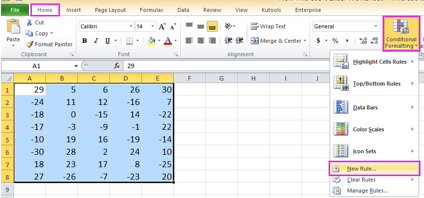
Go to the “Home” tab and click on “Conditional Formatting”.
Choose “Highlight Cells Rules” and select “More Rules”.
In the dialog box, choose “Format only cells that contain” under “Select a Rule Type”.
From the first drop-down menu, select “Specific Text”, then choose the desired cell color from the second drop-down menu.
Click “OK” to apply the formatting rule.

By applying this rule, all cells with the selected color will be highlighted automatically. To count them, use the following formula:

=COUNTIF(range,"*")

Replace range with your actual cell range.

Custom VBA Code Solutions

For more advanced users, custom VBA code can provide additional flexibility when counting colored cells in Excel. Here’s an example of how you can achieve this:

Function CountColoredCells(rng As Range) As Long
    Dim cel As Range
    Dim count As Long
    
    For Each cel In rng
        If cel.Interior.Color <> RGB(255, 255, 255) Then ' Change RGB values according to desired color
            count = count + 1
        End If
    Next cel
    
    CountColoredCells = count
End Function

To use this custom function, follow these steps:

Press ALT + F11 to open the Visual Basic Editor.
Insert a new module and paste the code provided.
Close the editor and return to your Excel worksheet.

The Power of Excel Formulas Based on Cell Color

We started by understanding the IF statement in Excel formulas, which allows you to perform conditional calculations based on cell color. Then, we delved into using the SUMIFS formula, which enables you to calculate sums based on specific cell colors. We learned how to apply the COUNTIF formula to count cells by color.

Moving forward, we explored different formulas for calculations based on cell color and discussed various methods to sum cells by color in Excel. Finally, we uncovered techniques for counting cells by color in Excel. By leveraging these powerful features and functions, you can enhance your data analysis capabilities and make more informed decisions.

If you want to take your Excel skills to the next level and unlock even more possibilities with formulas based on cell color, continue reading our future blog posts where we will dive deeper into advanced techniques and provide step-by-step tutorials. Stay tuned for more valuable insights that will help you become an Excel pro!

FAQs

Can I use formulas based on cell color in older versions of Excel?

Yes, formulas based on cell color are available in older versions of Excel as well. However, some specific functions or features may vary depending on the version you are using. It is recommended to consult the official documentation or online resources for compatibility information.

Are there any limitations when using formulas based on cell color?

While formulas based on cell color offer great flexibility and functionality, there are a few limitations to keep in mind. Firstly, they may not work properly if the workbook is opened in a different version of Excel that doesn’t support certain functions or features used in the formula. Secondly, changing or removing cell colors can affect the accuracy of these formulas if not updated accordingly.

Can I automate calculations based on changing cell colors?

Yes! You can automate calculations by using conditional formatting in conjunction with formulas based on cell color. By setting up rules for cell formatting, you can dynamically update the colors and trigger formula calculations automatically.

Is it possible to apply formulas based on font color or other cell attributes?

Yes, Excel allows you to apply formulas based on various cell attributes, including font color, fill pattern, and more. This gives you even more flexibility in your data analysis and decision-making processes.

Can I use formulas based on cell color in Excel Online or Google Sheets?

While Excel Online and Google Sheets offer similar functionalities as Microsoft Excel, the specific features and functions may vary slightly. It is recommended to consult the respective documentation or online resources for guidance on using formulas based on cell color in these platforms.