
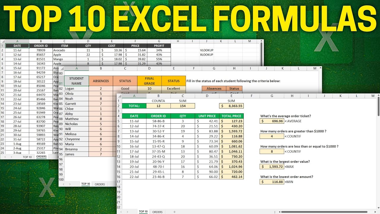
Excel formulas are a game-changer. Whether you’re a student, professional, or simply someone who deals with numbers on a regular basis in MS Excel, mastering mathematical operations and excel functions can significantly boost your productivity when working with numbers on an Excel sheet. That’s why we’ve compiled the top 10 Microsoft Excel formulas, including the vlookup function and mathematical operations, for everyday use. These formulas can be used to perform calculations using cell references and across different sheets.
=VLOOKUP(A2, B2:F100, 3, FALSE)
From basic calculations to advanced data manipulation, these excel functions have become an integral part of countless MS Excel workflows. Whether you’re working with a simple excel sheet or taking an excel course, mastering these formulas is essential. In this blog post, you’ll learn important excel formulas, including basic excel formulas and the vlookup formula. You’ll discover how to enter and reference arguments, use criteria to filter data, and even utilize the powerful INDEX function in the formulas tab.
=INDEX(A1:C10, MATCH(B2, A1:A10, 0), 3)
So if you’re looking to enhance your Excel skills and unlock the full potential of this widely used software, look no further! With the formulas tab, you can easily enter and manipulate data in your sheet using the vlookup formula. Get ready to enter practical examples and gain the knowledge needed to excel in any field. A2, the result of your efforts will be evident. Fig, dive in and start learning now!
Grasping Excel’s Fundamental Formulas
Basic Arithmetic Operations
To become proficient in Microsoft Excel, it is essential to understand the basic arithmetic operations, such as using formulas to calculate numbers and finding the sum of values. Additionally, learning how to use VLOOKUP can greatly enhance your Excel skills. These operations include addition, subtraction, multiplication, and division. With these formulas, such as vlookup and sum, at your disposal, you can easily perform simple calculations within Excel to obtain the desired number or result.
=SUM(A1:A10)
=A2+B2
=A2-B2
=A2*B2
=A2/B2
Cell References and Calculations Across Multiple Cells
One of the key features of Excel is its ability to perform calculations across multiple cells using cell references and formulas. With Excel, you can easily create a formula in a specific column, such as A1, and apply it to the entire table. This allows for efficient and accurate calculations throughout the entire spreadsheet. By using the advanced Excel function, you can create dynamic calculations that update automatically when the referenced cell values in a specific column of a table change. This allows for efficient data analysis and manipulation.
=SUM(A1:A10)
=AVERAGE(B1:B10)
Absolute and Relative Cell References
Excel offers two types of cell references: absolute and relative. The formula in cell A2 can be used to create a table. For example, when using the formula in cell A2, you can create a table. Absolute cell references are important excel formulas that remain fixed regardless of where the formula is copied or moved within a spreadsheet. This is a basic excel function that is widely used in advanced excel. On the other hand, when using basic Excel formulas, relative cell references in an Excel function will automatically adjust based on their new position when copied or moved within a table. This is a fundamental concept in advanced Excel functionality. Understanding the syntax of an Excel function is crucial for creating complex formulas that adapt to changes in data. Knowing how to reference a number or cell correctly is essential for this process.
Absolute Reference: =$A$1
Relative Reference: =A1
Common Mathematical Functions
In addition to basic arithmetic operations, Excel provides a wide range of mathematical functions that simplify complex calculations. With the help of these functions, you can easily perform various mathematical operations on numbers in different cells of your spreadsheet. This formulaic approach allows you to manipulate and analyze data efficiently. So, whether you need to perform a simple calculation or work with complex formulas, Excel’s mathematical functions have got you covered. Some common mathematical functions in Excel formulas include SUM, AVERAGE, MAX, and MIN. These functions allow you to quickly calculate the sum, average, maximum value, and minimum value from a range of cells. For example, you can use the SUM formula to get the result of adding a series of numbers together.
=SUM(A1:A10)
=AVERAGE(A1:A10)
=MAX(A1:A10)
=MIN(A1:A10)
Controlling Order of Operations with Parentheses
When working with complex formulas in Excel, understanding the syntax and order of operations is crucial to getting the desired result. Each number and cell must be placed correctly to ensure accurate calculations. Parentheses play a vital role in controlling the order of syntax in excel formulas by specifying which calculations should be performed first. This is important to ensure that the correct number is used, and to obtain the desired result. By using parentheses effectively in your formulas, you can ensure accurate results and avoid errors caused by incorrect calculation sequences. For example, if you want to calculate a syntax error or a number that requires a specific sequence, you can enter the necessary values within parentheses to prioritize their calculation.
=(A1 + B1) * (C1 - D1)
By mastering these fundamental concepts and techniques in Excel’s formula creation process, you will gain confidence in your ability to efficiently handle various data analysis tasks. For example, when working with Excel, you can enter formulas in a cell and see the result instantly.
Remember that practice makes perfect! To further enhance your Excel skills, consider enrolling in an advanced Excel course. Take advantage of online resources to enter formulas into cells. For example, you can learn how to use the formula bar to enter formulas into specific cells. The more you work with Excel and explore its features, the more comfortable you will become in using formulas to manipulate and analyze data in cells. This will result in a better understanding of how to enter formulas and analyze data using the cell functions available in Excel.
Mastering Text Manipulation with Excel Functions
Combine Text with CONCATENATE Function
The CONCATENATE formula in Microsoft Excel allows you to merge text from different cells into a single string. This formula is used to combine multiple strings together, resulting in a combined string. For example, you can use this formula to merge the contents of cell A1 and cell B1 into one string. The CONCATENATE function works with both text and number values, allowing you to merge different types of data. For example, if you have a first name in cell A1 and a last name in cell B1, you can use the CONCATENATE function in Excel formulas to combine them into one cell. This will give you a single cell with the combined first name and last name. This is particularly useful when working with large datasets or creating reports that require consolidated information. For example, in Excel formulas, you can use the SUM function to calculate the total of a range of cells. In Fig 1, you can see an example of how the SUM formula is used to add up the values in cell A1 to A5.
=CONCATENATE(A1, " ", B1)
Extract Specific Characters with LEFT, RIGHT, and MID Functions
Excel provides three functions – LEFT, RIGHT, and MID – that allow you to extract specific characters or substrings from a text string. These functions are useful when you need to manipulate data in a cell. For example, you can use the LEFT function to extract the first few characters from a cell, or the RIGHT function to extract the last few characters. The MID function allows you to extract a specific number of characters from a cell, starting from a specified position. In Figure 1 below, you can see an example of how these functions can be used in Excel. The LEFT formula extracts characters from the left side of a string, while the RIGHT formula does the opposite by extracting characters from the right side. For example, in a given number or cell, the LEFT function can be used to extract characters from the left side of the string. Similarly, the RIGHT function can be used to extract characters from the right side. The MID formula allows you to extract a substring by specifying the starting position and length. For example, in fig 1, the MID function is used to extract a specific number of characters from a cell. These functions are handy when dealing with data that requires parsing or extracting specific information. For example, if you have a large dataset and need to extract certain values from it, you can use formulas or functions in a spreadsheet program like Excel. By using the appropriate formula, you can easily retrieve the desired information from a specific cell or range of cells. This allows for efficient data analysis and manipulation.
=LEFT(A1, 3)
=RIGHT(A1, 2)
=MID(A1, 2, 3)
Convert Text Case with UPPER, LOWER, and PROPER Functions
To manipulate text case in Excel, you can utilize three functions: UPPER, LOWER, and PROPER. These functions allow you to change the case of a cell’s content. For example, if a cell contains a number, you can use the formula to convert it into uppercase or lowercase. The UPPER formula converts all letters in a text string to uppercase. For example, if you have a cell containing a lowercase word or number, you can use the UPPER function to convert it to uppercase. Conversely, the LOWER function converts all letters to lowercase. The PROPER formula is used to capitalize the first letter of each word in a text string. This can be seen in the example below. By applying the PROPER formula to a cell, all other letters in the text string will be converted to lowercase. See fig 1 for an illustration. These formula functions are valuable for standardizing data or formatting text based on specific requirements. For example, you can use the CELL function to retrieve information about a specific cell in a worksheet. Fig 1 shows an example of how to use this function.
- UPPER Function:
- Purpose: Converts all letters in a text string to uppercase.
- Example: If the cell A1 contains the text “excel functions”, the formula
=UPPER(A1)will return “EXCEL FUNCTIONS”.
- LOWER Function:
- Purpose: Converts all letters in a text string to lowercase.
- Example: If the cell A1 contains the text “EXCEL FUNCTIONS”, the formula
=LOWER(A1)will return “excel functions”.
- PROPER Function:
- Purpose: Converts the first letter of each word in a text string to uppercase and all other letters to lowercase.
- Example: If the cell A1 contains the text “eXcel funCtions”, the formula
=PROPER(A1)will return “Excel Functions”.
Powerful Text Manipulation Tools: REPLACE and SUBSTITUTE Functions
In Excel, there are two robust functions, REPLACE and SUBSTITUTE, for advanced text manipulation. These functions allow you to modify the content of a cell by replacing or substituting specific characters or strings. For example, you can use the REPLACE formula to change a specific part of a cell’s content, or the SUBSTITUTE formula to replace all occurrences of a word or phrase within a cell. Fig 1 shows an example of how these functions can be used in Excel. The REPLACE formula allows you to replace characters within a given text string based on their position and length parameters. This can be done by specifying the number of the fig cell where the replacement should occur. On the other hand, the SUBSTITUTE function is a formula that replaces specified occurrences of a particular character or substring within a cell’s text string with another character or substring of your choice. It is a useful tool for manipulating numbers and performing calculations.
- REPLACE Function:
- Purpose: Replaces part of a text string, based on the number of characters you specify, with a different text string.
- Example: If cell A1 contains the text “HelloWorld”, and you want to replace “World” with “Excel”, you would use the formula
=REPLACE(A1, 6, 5, "Excel"). This formula starts at the 6th character of “HelloWorld”, replaces the next 5 characters (“World”), resulting in “HelloExcel”.
- SUBSTITUTE Function:
- Purpose: Replaces existing text with new text in a text string. It replaces all occurrences of a specified substring.
- Example: If cell A1 contains “Apples and bananas”, and you want to replace all occurrences of “a” with “o”, you would use
=SUBSTITUTE(A1, "a", "o"). This changes “Apples and bananas” to “Opples ond bononos”.
These formula functions are extremely useful when cleaning up data or making specific changes to text strings in a cell. The number of these functions is quite impressive, and they can be used to manipulate data in various ways. For example, you can use the formula function to convert a text string into a number in a cell, or vice versa. Additionally, the formula function can be used to calculate the sum, average, or other mathematical operations on a range of numbers in a cell. In fig. 1 below, you can see an example of how the formula function is used to calculate For example, if you have a dataset with misspelled words or inconsistent formatting, the REPLACE and SUBSTITUTE functions can help you rectify these issues efficiently using a formula.
Custom Formatting with TEXT Function
The TEXT formula in Excel provides a powerful tool for custom formatting of dates, numbers, and more. With this formula, you can easily format your data to display exactly as you want it to. Whether you need to format a date as “mm/dd/yyyy” or a number as currency with two decimal places, the TEXT formula has got you covered. It’s like having a fig at your fingertips, allowing you to mold your data into the perfect shape. So if you’re tired of struggling with formatting in Excel, give the TEXT formula a try and see how it can simplify your life This formula function allows you to convert values into specific formats according to your requirements. Using this function, you can easily manipulate and transform data using a simple formula. Whether you need to convert units, calculate percentages, or perform complex mathematical operations, this formula function has got you covered. With just a few clicks, you can apply the desired format to your data and obtain the results you need. So, don’t waste time manually converting values – let this formula function do the work for you. For instance, if you have a date value that is displayed as “2022-01-01” but want it to appear as “January 1, 2022,” the TEXT formula can accomplish this transformation.
By combining the TEXT formula with various formatting codes, you can achieve precise control over how data is presented in your spreadsheets. Using the formula, you can format the data to appear in a specific way, such as displaying it as a currency or as a percentage. This gives you the flexibility to customize the appearance of your data to suit your needs. With the help of the formula, you can create professional-looking spreadsheets that are easy to read and understand. So, whether you want to display numbers as fractions or add leading zeros to your text, the TEXT formula is the key to achieving the desired formatting. This flexibility is particularly valuable when working with complex datasets or when generating reports that require specific formatting. It allows you to easily incorporate formulas, figures, and functions into your work.
Calculating and Summarizing Data Efficiently
Utilize COUNT function to count the number of cells containing values within a range.
The COUNT formula in Microsoft Excel is a powerful tool that quickly determines the number of cells containing values within a specified range. This can be incredibly useful when you need to keep track of data or perform calculations based on the presence or absence of certain values within a function. By using the COUNT function, you can easily identify how many items meet specific criteria without having to manually count them one by one.
For example, let’s say you have a list of sales figures for different products in column A, and you want to know how many products have sold more than 100 units. In this case, you can use the “COUNTIF” function to easily count the number of products that meet this criteria. By applying the COUNT function with the condition “>100” to the range of sales figures, Excel will instantly provide you with the total count of products meeting this criterion.
Learn how to calculate percentages using simple division or percentage-specific functions like PERCENTAGE or PERCENTRANK.
Calculating percentages is a common function in Excel, whether it’s determining growth rates, analyzing survey responses, or comparing data sets. There are multiple ways to calculate percentages in Excel, depending on your specific needs. One of the most useful functions in Excel is the percentage function, which allows you to easily calculate percentages.
One straightforward method involves using a mathematical function by dividing one value by another and multiplying by 100. For instance, if you want to find out the percentage of 75 in 1000, use the divide function to divide 75 by 1000 (0.075) and then multiply by 100 using the multiply function to get the result (7.5%). This basic formula can be applied in various scenarios where percentages need to be calculated. It is a versatile function that can be used in different contexts.
- Calculating Percentage:
- Method: Divide the part by the whole and then multiply by 100 to get a percentage.
- Example: If you want to find out what percentage 50 is of 200, you would use the formula
=50/200*100. This will give you 25%, indicating that 50 is 25% of 200.
- PERCENTRANK Function:
- Purpose: Returns the rank of a value in a data set as a percentage (0..1) of the data set.
- Example: Suppose you have a list of numbers in cells A1 through A10 and you want to find the percentile rank of the value in A5. You would use
=PERCENTRANK(A1:A10, A5). This will return the percentile rank of the value in A5 compared to the other values in the range A1 through A10.
Excel offers specialized functions like PERCENTAGE and PERCENTRANK that simplify percentage calculations further. The PERCENTAGE function allows you to convert a decimal value into a percentage format directly. On the other hand, the PERCENTRANK function calculates the rank percentile position for a given value within a dataset as a percentage.
Discover the power of SUMIF function for conditional summing based on specific criteria.
The SUMIF function is an invaluable tool. The function allows you to add up values from a range that meet specific criteria or conditions. This can be particularly useful when dealing with large data sets and you want to extract specific information based on certain conditions using a function.
For example, suppose you have a table containing sales data for different products, and you want to calculate the total revenue generated by a particular product category using a function. By using the SUMIF function with the condition “Product Category = Electronics,” Excel will automatically sum up all the sales figures for electronics products, providing you with the desired result.
Explore AVERAGEIF function for calculating averages based on specified conditions.
Similar to the SUMIF function, Excel’s AVERAGEIF function allows you to calculate averages based on specified conditions. This function can be helpful when you need to selectively analyze data and determine average values for specific subsets of your dataset.
For instance, let’s say you have a table with student scores in different subjects, and you want to find out the average score for students who scored above 80 in a particular subject using a function. By utilizing the AVERAGEIF function with the condition “Subject = Math” and “Score > 80,” Excel will calculate the average score specifically for those students who meet these criteria.
Master pivot tables for quick data summarization and analysis.
Pivot tables are a powerful function in Microsoft Excel that allow you to quickly summarize and analyze large amounts of data. They enable users to transform raw data into meaningful insights without complex formulas or manual calculations using the function.
By using pivot tables, you can easily group, filter, sort, and summarize data based on various parameters such as categories or time periods. This is made possible through the use of the function. They provide dynamic views of your dataset that can be adjusted instantly as per your function requirements. Whether it’s analyzing sales figures by region or examining survey responses by age group, pivot tables function as a versatile and efficient way to gain valuable insights from your data.
Making the Most of Lookup and Reference Functions
VLOOKUP: Retrieving Data with Ease
The VLOOKUP function in Microsoft Excel is a powerful tool that allows you to quickly retrieve data from a table based on a specified lookup value. The function saves time and effort by automating the process of searching for information in large datasets. With the VLOOKUP function, you can easily find relevant data by specifying the lookup value and selecting the appropriate column to search within.
HLOOKUP: Looking Horizontally
While VLOOKUP is useful for vertical lookups, Excel also offers the HLOOKUP function for horizontal lookups. With the HLOOKUP function, you can search for data across rows instead of columns. This function comes in handy when working with datasets organized horizontally or when you need to extract specific information from a row.
INDEX and MATCH: Flexibility and Power Combined
Combining the INDEX and MATCH functions can be incredibly beneficial. The INDEX function allows you to return a value from an array based on its position, while the MATCH function helps locate the position of a specified value within an array. By using these two functions together, you can perform complex lookups that are not possible with VLOOKUP or HLOOKUP alone.
INDIRECT: Indirectly Referring to Cells or Ranges
The INDIRECT function in Excel provides another level of flexibility by allowing you to refer to cells or ranges indirectly. Instead of directly referencing a cell or range, you can use the INDIRECT function to refer to them indirectly by providing their address as text within the formula. This function becomes particularly useful when dealing with dynamic formulas that need to adjust automatically based on changing conditions.
OFFSET: Dynamic Referencing Made Easy
Excel’s OFFSET function enables dynamic referencing by allowing you to reference cells or ranges that are offset from a starting point. You specify the starting cell in the function, the number of rows and columns to offset, and the size of the range you want to return. This function is especially handy when you need to create formulas that adapt to changes in your data, as it automatically adjusts the referenced cells or ranges based on the specified offset.
By mastering these lookup and reference functions in Microsoft Excel, you can significantly enhance your data analysis capabilities. Whether you’re retrieving specific information from large datasets or creating dynamic formulas that adapt to changing conditions, these functions provide the flexibility and power needed for everyday use.
Remember, practice makes perfect. Take some time to experiment with these functions and explore their various applications. The more familiar you become with the function, the more efficiently you’ll be able to work with Excel and make the most of its features.
Organizing and Cleaning Data with Excel
Use Data Validation for Controlled Data Entry
Data validation is a powerful function in Microsoft Excel that allows you to set restrictions on the type of data entered into specific cells or ranges. By utilizing data validation, you can ensure that the inputted data meets certain criteria, such as numerical values within a specified range or selecting from a predefined list. This ensures that the function of the data is optimized and accurate. This function helps maintain data integrity and reduces errors in your Excel sheet.
Remove Duplicates for Clean Data Sets
When working with large datasets, it’s common to encounter duplicate entries. This is where the function comes into play. However, having duplicate data can negatively impact the accuracy of analysis and distort the results of a function. Thankfully, Excel provides built-in tools to help you remove duplicates effortlessly using its function. By identifying and eliminating duplicate values, you can streamline the function of your data and ensure its accuracy.
Highlighting Patterns with Conditional Formatting
Conditional formatting is a function in Excel that allows you to visually highlight specific patterns or values in your dataset. It is an invaluable tool. With conditional formatting, you can apply different formatting styles based on certain conditions or rules that you define using the function. This function enables you to draw attention to important trends or outliers within your data, making it easier to analyze and interpret.
Sorting and Filtering for Effective Organization
Excel offers a variety of functions, including robust sorting and filtering options, that allow you to effectively organize your data. Sorting is a fundamental function that allows you to arrange your data in either ascending or descending order, depending on specific columns or criteria. On the other hand, the filtering function allows you to display only the relevant information by hiding rows that do not meet certain conditions. These features function to enable quick access to the desired information while maintaining the overall structure and function of your spreadsheet.
Splitting Data using Text-to-Columns Feature
Sometimes, when dealing with large amounts of text in a single column, it becomes necessary to split it into separate columns based on delimiters (such as commas or spaces) using a function. The function of the text-to-columns feature in Excel simplifies this process by automatically separating text into multiple columns based on the chosen delimiter. This functionality is particularly useful when dealing with datasets that require further analysis or manipulation.
By utilizing the powerful function features, you can effectively organize and clean your data in Microsoft Excel. Whether you need to control data entry, remove duplicates, highlight patterns, or sort and filter information, Excel provides the necessary tools to simplify these tasks with ease and efficiency. With its robust function capabilities, Excel empowers users to streamline their data management processes. With a well-organized spreadsheet and clean dataset, you can enhance the function of your analysis and make more informed decisions based on accurate information.
Harnessing the Power of Date and Time Functions
Understand Excel’s Numeric Representation of Dates and Times
Excel functions treat dates and times as numeric values, enabling powerful calculations and manipulations. Each date is assigned a unique serial number using the function, with January 1, 1900, having the value 1. By understanding this numeric representation, you can leverage Excel’s built-in functions to perform various operations on dates and times.
Calculate Time Differences with Ease
Whether you need to determine the duration between two time points or calculate working days excluding weekends and holidays, Excel offers several function methods. The function of simple subtraction can be used to find the time difference between two cells containing time values. However, specialized functions like DATEDIF or NETWORKDAYS.INTL provide more flexibility in calculating precise differences based on specific criteria.
Utilize Date-Specific Functions for Versatile Calculations
Excel provides a range of date-specific functions that simplify complex calculations involving dates. The TODAY function returns the current system date, allowing you to create dynamic formulas that automatically update with each passing day. The NOW function provides both the current date and time information.
Functions like DATE, YEAR, MONTH, DAY enable extracting specific components from a given date value. For example, you can use these functions to extract the year from a birthdate column or determine the month of an invoice due date.
Extract Specific Components from Time Values
Similar to date-specific functions, Excel also offers time-specific functions that allow you to extract specific components from time values. HOUR extracts the hour component from a given time value while MINUTE retrieves minutes and SECOND retrieves seconds. These functions are particularly useful when analyzing datasets that involve timestamps or tracking durations.
Master Conditional Formatting Techniques Based on Date Criteria
Conditional formatting is a powerful feature in Excel that allows you to format cells based on specified criteria.Conditional formatting can be used effectively to highlight upcoming deadlines or identify overdue tasks. By applying formatting rules based on date criteria, you can quickly visualize and prioritize important dates in your data.
For example, you can use conditional formatting to highlight all dates that are within a certain number of days from the current system date. This visual cue helps in identifying approaching deadlines or events at a glance.
Utilizing Logical and Conditional Formulas
Logical Operators for Complex Tests
In Excel, you can create complex logical tests by using logical operators such as AND, OR, and NOT in conjunction with the IF function. These operators allow you to evaluate multiple conditions simultaneously and make decisions based on the results. For example, you can use the AND operator to check if two or more conditions are true before executing a specific action. Similarly, the OR operator allows you to perform an action if at least one of the conditions is true. On the other hand, the NOT operator helps you negate a condition, allowing you to execute an action when a particular condition is false.
Nested IF Statements for Multiple Conditions Evaluation
When dealing with multiple conditions in Excel formulas, nested IF statements come in handy. This technique involves embedding one IF statement within another to evaluate different scenarios based on various conditions. By nesting IF statements together, you can create sophisticated decision-making formulas that cater to specific requirements. Each nested IF statement acts as an alternative branch of logic within the formula, allowing for intricate calculations and data manipulations.
Counting Cells Meeting Specific Criteria
The COUNTIF function is a powerful tool for counting cells that meet specific criteria in Excel. With this formula, you can easily determine how many cells in a range satisfy certain conditions. The COUNTIF function requires two arguments: the range of cells to be evaluated and the criteria that need to be met for inclusion in the count. By utilizing numerical values or equal signs along with wildcards like asterisks (*) or question marks (?), you can perform precise counts based on your specified criteria.
Summing Values Based on Multiple Conditions
The SUMIFS function enables you to sum values from a range based on multiple conditions simultaneously. This versatile formula allows you to specify different criteria across multiple columns and calculate their corresponding sums efficiently. By providing ranges for each criterion and their respective values, SUMIFS adds up the values that meet all the specified conditions. Whether you need to sum sales figures by region, product category, or any other combination of criteria, SUMIFS provides a straightforward solution.
Calculating Averages Based on Specified Conditions
Excel’s AVERAGEIFS function allows you to calculate averages based on specific conditions. Similar to SUMIFS, this formula enables you to define multiple criteria across different columns and calculate the average of corresponding values. By specifying ranges for each criterion and their respective conditions, AVERAGEIFS calculates the average of only those values that meet all the specified criteria. This functionality is particularly useful when you want to analyze data subsets and obtain average values based on specific filters or combinations of criteria.
Utilizing these logical and conditional formulas in Microsoft Excel can greatly enhance your ability to perform complex calculations, make data-driven decisions, and analyze information effectively. Whether you’re counting cells meeting specific criteria using COUNTIF, summing values based on multiple conditions with SUMIFS, or calculating averages using AVERAGEIFS, mastering these formulas will undoubtedly streamline your everyday use of Excel.
Remember to experiment with different scenarios and explore various combinations of logical operators and nested IF statements to fully leverage the power of these formulas. With practice and familiarity, you’ll become proficient in creating dynamic Excel formulas that cater precisely to your needs.
Simplifying Complex Calculations with Advanced Functions
Array Formulas: Performing Simultaneous Calculations
Array formulas are a powerful tool in Microsoft Excel that allow you to perform calculations across multiple cells simultaneously. By using an array formula, you can avoid the need for repetitive calculations and streamline complex tasks. For example, if you have a range of numbers and want to find their sum, you can use the SUM function as an array formula to calculate the sum of all the numbers in one go.
Financial Functions: Analyzing Financial Data
Microsoft Excel offers several useful functions that simplify complex calculations. The PMT (payment) function allows you to determine the fixed periodic payment required for a loan or mortgage. The FV (future value) function helps you calculate the future value of an investment based on regular contributions and interest rates. Similarly, the PV (present value) function assists in determining the present value of future cash flows.
Statistical Functions: Analyzing Data Trends and Relationships
Excel provides various statistical functions that aid in analyzing data trends and relationships. The AVERAGEIF function allows you to calculate the average of a range of values based on specified criteria. This is particularly useful when dealing with large datasets where specific conditions need to be met. The STDEV function calculates the standard deviation, which measures how much data varies from its mean value. The CORREL function determines the correlation coefficient between two sets of data, helping identify any relationship between them.
Mathematical Functions: Advanced Calculations Made Easy
Microsoft Excel includes a range of mathematical functions that facilitate advanced calculations. The POWER function enables you to raise a number to a specified power easily. For instance, if you want to calculate compound interest or exponential growth, this function will come in handy. The SQRT (square root) function finds the square root of a given number swiftly and accurately. Moreover, with the ABS (absolute) function, you can quickly obtain the absolute value of a number, regardless of its positive or negative sign.
INDEX and MATCH: Complex Data Retrieval
INDEX and MATCH are two powerful functions that work exceptionally well together for complex data retrieval. The INDEX function allows you to retrieve a value from a specified range based on its position within that range. On the other hand, the MATCH function helps locate the position of a specific value within a range. By combining these functions, you can perform dynamic lookups in your worksheets, making it easier to extract data from large datasets or create interactive reports.
By mastering these advanced functions in Microsoft Excel, you can simplify complex calculations and save valuable time. Whether you’re working with financial data, analyzing statistics, or performing mathematical calculations, utilizing these formulas will enhance your productivity and efficiency.
Tailoring Excel for Personalized Data Analysis
Custom Functions with VBA
Expand your Excel skills by learning how to create custom functions using VBA (Visual Basic for Applications). VBA allows you to extend Excel’s functionality beyond its built-in formulas. With custom functions, you can automate repetitive tasks, perform complex calculations, and manipulate data in unique ways. By writing your own code, you have the flexibility to tailor Excel to your specific needs.
Power of Pivot Charts
Discover the power of pivot charts for visualizing data trends and patterns. Pivot charts are a dynamic way to present your data visually, allowing you to analyze large datasets with ease. With just a few clicks, you can summarize and visualize your data in various chart types such as bar graphs, line graphs, and pie charts. Pivot charts enable you to gain valuable insights into your data and communicate them effectively.
Conditional Formatting Rules
Take advantage of conditional formatting rules in Excel to highlight specific data points based on user-defined criteria. Conditional formatting allows you to apply different formatting styles such as colors, icons, or data bars based on certain conditions. This feature is particularly useful when dealing with large datasets or when you want to draw attention to important information quickly. By setting up conditional formatting rules, you can easily identify outliers or spot trends within your data.
Sensitivity Analysis with Data Tables
Utilize data tables in Excel to perform sensitivity analysis by varying input values in a model. Sensitivity analysis helps assess how changes in variables impact the outcome of a calculation or model. With data tables, you can set up multiple scenarios by specifying different input values and instantly see how they affect the results. This feature is invaluable for financial analysis or any situation where understanding the impact of changing variables is crucial.
Goal Seek Feature
Find out how to use the goal seek feature in Excel to determine the input value needed to achieve a desired result. Goal seek allows you to work backward from a specific outcome and find the corresponding input value. This feature is particularly useful when you have a target in mind and need to determine the necessary input to reach that goal. Whether it’s finding the sales volume required to meet a revenue target or determining the interest rate needed for a desired loan payment, goal seek can save you time and effort.
Conclusion
Congratulations! You have now mastered the top 10 Microsoft Excel formulas for everyday use. By grasping the fundamental formulas, manipulating text efficiently, calculating and summarizing data effectively, utilizing lookup and reference functions, organizing and cleaning data effortlessly, harnessing the power of date and time functions, employing logical and conditional formulas, simplifying complex calculations with advanced functions, and tailoring Excel for personalized data analysis, you are well-equipped to tackle any spreadsheet challenge that comes your way.
Now it’s time to put your newfound Excel skills into action! Start applying these formulas in your daily work or personal projects. Whether you’re a student analyzing data for a research paper or a professional managing budgets and forecasts, Excel’s powerful formulas will save you time and effort. Remember to practice regularly to reinforce your understanding and explore additional resources to expand your Excel knowledge even further. With determination and practice, you’ll become an Excel expert in no time!
Frequently Asked Questions
FAQ
How can I grasp Excel’s fundamental formulas?
To grasp Excel’s fundamental formulas, start by familiarizing yourself with basic functions like SUM, AVERAGE, and COUNT. Practice using these functions on simple datasets to understand their purpose and how they work. As you gain confidence, explore more advanced formulas like IF statements and VLOOKUP to enhance your Excel skills.
What are some essential Excel functions for text manipulation?
Excel offers several powerful functions for text manipulation. CONCATENATE combines multiple strings into one, LEFT extracts a specified number of characters from the left side of a cell, and FIND locates the position of a specific character within a string. These functions enable you to manipulate and format text efficiently in Excel.
How can I calculate and summarize data efficiently in Excel?
Excel provides various functions to calculate and summarize data effectively. The SUM function adds up values in a range, while AVERAGE calculates the average value. MAX returns the highest value in a range, MIN returns the lowest value, and COUNT counts the number of cells containing numerical data.
What are lookup and reference functions in Excel used for?
Lookup and reference functions in Excel allow you to find specific information within large datasets. Functions like VLOOKUP help you search vertically for a value in one column based on another column’s corresponding value. INDEX-MATCH is another powerful combination that enables you to look up values horizontally or vertically.
How can I organize and clean data using Excel?
Excel offers various tools to organize and clean data efficiently. Use filters to sort data based on specific criteria or remove duplicates with the Remove Duplicates feature. You can also use Text-to-Columns to split data into separate columns based on delimiters or utilize conditional formatting to highlight inconsistencies or errors within your dataset.