Excel Formulas Date Range: Mastering & Ultimate Guide

In the world of Excel, mastering the art of formulas is essential for efficient data analysis and manipulation. With the help of charts and tools, you can visualize your data and gain valuable insights. If you’re new to Excel, don’t worry! Our tutorial will guide you step-by-step on how to use formulas effectively, starting with cell A2. With the help of charts and tools, you can visualize your data and gain valuable insights. If you’re new to Excel, don’t worry! Our tutorial will guide you step-by-step on how to use formulas effectively, starting with cell A2.

One area that often poses a challenge for users is working with date ranges. When it comes to working with start_date and sum_range, users may find it difficult to calculate the number of workdays using the right tools. When it comes to working with start_date and sum_range, users may find it difficult to calculate the number of workdays using the right tools. Understanding how to utilize date ranges in Excel formulas, such as sum_range, can greatly enhance your spreadsheet capabilities. By incorporating these tools, you can create dynamic charts and analyze data starting from a specific start_date.

Precision and accuracy are paramount. Whether you’re tracking project deadlines, analyzing sales trends over time, or calculating durations between two points, having a solid grasp on Excel formulas for date calculations is crucial.

These formulas can help you accurately calculate the number of workdays between a start_date and an end_date, making it easier to meet project criteria and deadlines. With the right tools and knowledge, you can efficiently perform these calculations in Excel. These formulas can help you accurately calculate the number of workdays between a start_date and an end_date, making it easier to meet project criteria and deadlines. With the right tools and knowledge, you can efficiently perform these calculations in Excel.

By utilizing the power of date ranges in your spreadsheets, you can maximize your productivity with the right tools and efficiently manage your workdays. Whether it’s calculating start_date for a project or utilizing formula examples to streamline your processes, the possibilities are endless. From performing complex calculations using date functions to generating dynamic reports based on specific time periods, Excel’s formula capabilities can streamline your workflow and save valuable time. Whether you need to calculate workdays or apply criteria to your data, Excel’s date functions can help. Here are some examples of how you can use date functions in Excel to enhance your productivity.

Understanding Date Formats in Excel

Familiarize yourself with different date formats in Excel

When working with dates in Excel, it is important to understand the various date formats that can be used in your workday. Here are some formula examples that can help you manipulate and format dates in Excel. By using these formulas, you can easily extract specific information from a date, such as the day, month, or year. Additionally, you can compare dates using criteria and perform calculations based on the date values. Understanding how to work with dates and apply the appropriate formulas can greatly enhance your Excel skills and make your workday more efficient. By familiarizing yourself with formula examples and text formats, you can ensure that your data in cell A2 is displayed correctly based on the given criteria and avoid any confusion.

Excel offers a wide range of built-in date formats, including short and long date formats, as well as custom formats. In addition, Excel provides formula examples for working with dates and times. You can use the WORKDAY function to calculate the workday after a given date, or the TEXT function to format a date in a specific way. For example, you can use the A2 cell reference in your formula to perform calculations based on the value in that cell. In addition, Excel provides formula examples for working with dates and times. You can use the WORKDAY function to calculate the workday after a given date, or the TEXT function to format a date in a specific way. For example, you can use the A2 cell reference in your formula to perform calculations based on the value in that cell. Short date formats typically display the day, month, and year (e.g., 12/31/2022), while long date formats may include the day of the week (e.g., Friday, December 31, 2022). In a2, you can use formula examples to format dates based on specific criteria. In a2, you can use formula examples to format dates based on specific criteria. Custom formats, such as formula examples, allow you to specify a format based on specific criteria. For instance, you can use the formula in cell A2 and apply it to cell C2.

To apply a specific date format to a cell or range of cells in Excel, follow these steps. Use the formula examples to format the day in cell A2 based on the given criteria.

1. Select the cell(s) where you want to apply the format using formula examples. Use excel date functions and criteria in the selected cell(s), such as A2.

2. Right-click and choose “Format Cells” from the context menu for excel date functions.

3. In the Format Cells dialog box, navigate to the “Number” tab for excel date functions. Use formula examples like A2 and C2.

4. Select “Date” from the Category list on the left.

5. Choose your desired format from the list or customize it using the options provided. You can use formula examples and criteria to customize the format. For example, you can use the formula “a2” to specify the criteria for customizing the format. This will ensure that the customized format returns the desired results. You can use formula examples and criteria to customize the format. For example, you can use the formula “a2” to specify the criteria for customizing the format. This will ensure that the customized format returns the desired results.

6. Click “OK” to apply the format.

Learn how to change the default date format in Excel

By default, Excel uses a specific date format based on your computer’s regional settings. However, you can customize the format using formula examples. For example, if you want to display the date in cell A2 in a different format, you can use the formula =TEXT(A2, “dd/mm/yyyy”). Similarly, if you want to convert a text string in cell C2 into a date format, you can use the formula =DATEVALUE(C2). Additionally, if you want to determine if a date in cell C10 is a weekday or weekend, you can However, you can customize the format using formula examples. For example, if you want to display the date in cell A2 in a different format, you can use the formula =TEXT(A2, “dd/mm/yyyy”). Similarly, if you want to convert a text string in cell C2 into a date format, you can use the formula =DATEVALUE(C2). Additionally, if you want to determine if a date in cell C10 is a weekday or weekend, you can However, if you prefer a different default date format for your workbooks or want consistency across multiple computers, you can modify this setting. For example, you can use formula examples like =A2+C2-C10 to customize the date format. For example, you can use formula examples like =A2+C2-C10 to customize the date format.

To change the default date format in Excel:

1. Click on “File” in the top left corner of Excel to access formula examples.

2. Select “Options” from the dropdown menu.

3. In the Excel Options dialog box, click on “Advanced.”

4. Scroll down until you find “When calculating this workbook.”

5. Modify the “Use this date format” field to your desired format, which can include formula examples and c10. This modification will ensure that the field returns the desired results.

6. Click “OK” to save the changes.

By changing the default date format, you can ensure that any new workbooks you create in Excel will automatically use your preferred format for returns and c10.

Understand how to customize date formats based on your needs

Excel provides a powerful feature that allows you to customize date formats according to your specific needs and returns. This flexibility enables you to display dates in various ways, such as showing only the month and year or including additional information like the day of the week. With this feature, you can easily customize the returns of date formats to suit your needs. With this feature, you can easily customize the returns of date formats to suit your needs.

To customize a date format in Excel:

1. Select the cell(s) containing the dates you want to format.

2. Right-click and choose “Format Cells.”

3. In the Format Cells dialog box, go to the “Number” tab.

4. Select “Custom” from the Category list.

5. In the Type field, enter a custom format code using a combination of letters and symbols.

   • For example, “mm/dd/yyyy” displays dates as 01/31/2022.

   • To include the day of the week, use “dddd mm/dd/yyyy,” which shows dates like Monday 01/31/2022.

6. Preview your changes in the Sample section.

7. Click “OK” when satisfied with your custom format.

Experimenting with different custom formats allows you to tailor Excel’s date representation precisely according to your preferences and requirements.

Typing Start and End Dates in Excel

Shortcuts for Quick Date Entry

Mastering the art of shortcuts can be a game-changer. Instead of manually inputting each date, you can save time by using these handy tricks:

1. AutoFill: If you have a series of dates with a consistent pattern (e.g., daily, weekly, monthly), simply enter the start date and drag the fill handle down or across to automatically populate the remaining dates.

2. Keyboard Shortcuts: Excel offers several keyboard shortcuts for quickly typing specific types of dates. For example:

   • To enter today’s date: Press Ctrl + ; (semicolon).

   • To enter the current time: Press Ctrl + Shift + ; (semicolon).

3. Relative Dates: When working with relative dates, such as “30 days from today” or “next Monday,” you can use formulas like TODAY(), NOW(), and functions like EDATE() or EOMONTH() to calculate the desired date dynamically.

Handling Different Date Separators and Formats

In Excel, it’s essential to understand how to handle different date separators and formats while typing. Here are some tips to ensure accuracy:

1. Date Separators: Excel supports various date separators, including slashes (/), dashes (-), periods (.), and even spaces. However, it’s crucial to use a consistent separator throughout your data entry process for better readability.

2. Regional Settings: Depending on your regional settings, Excel may interpret certain date formats differently. For example, in some regions, “03/04/2022” represents March 4th, while in others it denotes April 3rd. To avoid confusion, consider using the universal format (YYYY-MM-DD) or adjusting your regional settings accordingly.

3. Text to Columns: If you have a large dataset with dates in different formats, Excel’s “Text to Columns” feature can help. Select the column containing the dates, go to the “Data” tab, click on “Text to Columns,” and follow the wizard to specify the delimiter and date format.

Avoiding Errors with Large Date Sets

When dealing with sizable sets of dates, it’s easy to make mistakes that could lead to incorrect calculations or data inconsistencies. Here are techniques for error prevention:

1. Data Validation: Implement data validation rules for your date columns. You can set criteria such as allowing only specific date ranges or preventing duplicate entries. This helps maintain data integrity and prevents accidental errors.

2. Paste Special: When copying and pasting dates from external sources into Excel, be cautious about preserving their original formatting. To avoid any issues, use the “Paste Special” feature (right-click > Paste Special) and select “Values” or “Match Destination Formatting.”

3. Conditional Formatting: Apply conditional formatting rules to highlight potential errors in your date columns automatically. For instance, you can create a rule that flags any date earlier than today or any duplicated dates within a range.

Creating Dynamic Date Ranges

Unlock the power of dynamic date ranges using formulas in Excel. With these flexible formulas, you can save time and effort by automatically updating your data based on current dates. Let’s dive into the world of dynamic date ranges and explore various functions that make generating start and end dates effortless.

Generate Start and End Dates Automatically

One of the key benefits of using Excel formulas for date ranges is the ability to generate start and end dates automatically. By leveraging specific functions, you can ensure that your date range always reflects the current period.

To create a dynamic start date, you can use the TODAY function. This function returns today’s date, which means it will update every time you open or recalculate your spreadsheet. For example:

=TODAY()

Similarly, to generate an automatic end date, you can combine the TODAY function with other functions like EOMONTH (End Of Month). EOMONTH returns the last day of a specified month based on a given date. Here’s an example:

=EOMONTH(TODAY(), 0)

With these formulas in place, your start and end dates will always adjust accordingly without any manual intervention.

Adjust Dynamic Ranges Based on Specific Criteria

Excel also allows you to adjust dynamic ranges based on specific criteria or conditions. This feature is particularly useful when dealing with large datasets or when you want to focus on a subset of information within your date range.

To accomplish this, you can utilize functions like IF and COUNTIFS together with your dynamic range formula. For instance, if you only want to include data from a certain category within your dynamic range, consider using an IF statement combined with COUNTIFS:

=IF(COUNTIFS(CategoryRange,"CategoryName",DateRange">="&StartDate,"DateRange"<="&EndDate)>0,[DataRange],"")

This formula checks if the category matches your specified criteria and falls within the desired date range. If it does, it includes the corresponding data; otherwise, it returns an empty cell.

Advanced Techniques for Complex Dynamic Date Ranges

Excel offers advanced techniques to create even more complex dynamic date ranges. These techniques involve combining multiple functions and logical operators to meet specific requirements.

For example, you can use the NETWORKDAYS.INTL function to calculate the number of working days between two dates while excluding weekends and custom holidays. This is especially helpful when dealing with project timelines or tracking employee attendance.

Another powerful function is SUMIFS, which allows you to sum values based on multiple criteria. By incorporating this function into your dynamic date range formula, you can perform calculations on specific data within a given period.

=SUMIFS(DataRange,DateRange,">="&StartDate,DateRange,"<="&EndDate,CriteriaRange,"Criteria")

In this formula, DataRange represents the values you want to sum, DateRange is the range containing your dates, StartDate and EndDate define your desired period, and CriteriaRange determines additional conditions for selecting specific data.

By exploring these advanced techniques and experimenting with different combinations of functions, you can create highly customized dynamic date ranges that cater to your unique needs in Excel.

Calculating Date Differences

Master the art of calculating differences between two dates in Excel formulas. We will delve into practical examples showcasing the applications of calculating date differences and provide tips on formatting calculated results as desired.

Understanding Date Functions

Understanding the available date functions is crucial. These functions enable us to perform calculations involving dates efficiently. One such function is the EDATE function, which allows us to add or subtract a specified number of months from a given date. By utilizing this function, you can easily calculate future or past dates based on your requirements.

Calculating Time Intervals

To calculate the difference between two dates accurately, Excel provides several functions that cater to different scenarios. The DATEDIF function is particularly useful when you need to determine the number of days, months, or years between two dates. This versatile function allows you to specify the unit of measurement (days “d,” months “m,” or years “y”) and returns the corresponding value.

For instance, suppose you want to find out how many days have passed since a particular event occurred until today’s date. You can use the DATEDIF function by subtracting the earlier date from today’s current date:

=DATEDIF(start_date,TODAY(),"d")

By replacing start_date with your desired start date in cell reference format (e.g., A1), this formula will give you an accurate count of elapsed days.

Leap Years and Beyond

Calculating date differences becomes more intricate when leap years come into play. Leap years consist of 366 days instead of 365 due to an extra day added in February every four years. To ensure precise calculations that account for leap years, you can combine the DATEDIF function with other date functions like YEAR and MONTH. By extracting the year and month components from each date, you can accurately calculate differences while considering leap years.

For example, let’s say you want to find the number of months between two dates, accounting for leap years. You can use the following formula:

=DATEDIF(start_date,end_date,"m") + 12 * (YEAR(end_date) - YEAR(start_date)) + MONTH(end_date) - MONTH(start_date)

By substituting start_date and end_date with your desired dates in cell references, this formula will provide an accurate count of months between the two dates, even if they span multiple years.

Practical Applications

Calculating date differences finds practical applications in various scenarios. For instance, it can be useful in tracking project durations or determining employee tenures. By utilizing Excel formulas to calculate these differences automatically, you can save time and effort.

Suppose you have a list of project start dates in column A and end dates in column B. To calculate the duration of each project automatically, you can use the following formula in column C:

=DATEDIF(A2,B2,"d")

This formula calculates the number of days between each start and end date, providing valuable insights into project timelines.

Working with Week Numbers and Weekdays

Understand how week numbers are used in relation to calendar weeks

Week numbers are a useful way to organize and track time, especially when working with large datasets or planning projects. In Excel, week numbers follow the ISO 8601 standard, where each year has 52 or 53 weeks. This standard ensures consistency across different countries and regions.

When dealing with week numbers, it’s essential to understand their relationship to calendar weeks. The first week of the year is the one that contains at least four days of January. For example, if January 1st falls on a Wednesday or earlier, then the first week starts on January 1st. However, if January 1st is a Thursday or later, then the first week begins on the following Monday.

Learn about Excel functions for extracting week numbers and weekdays from dates

Excel provides several powerful functions for extracting week numbers and weekdays from dates. These functions allow you to perform various calculations based on specific timeframes.

To extract the week number from a date in Excel, you can use the WEEKNUM function. This function takes a date as input and returns the corresponding week number based on your chosen system (e.g., starting from Sunday or Monday).

For example, suppose you have a date in cell A2 that corresponds to May 15th, 2022. You can use the formula =WEEKNUM(A2) to retrieve the week number associated with that date.

Similarly, if you need to determine the weekday (e.g., Monday, Tuesday) of a particular date in Excel, you can utilize the WEEKDAY function. This function allows you to specify whether weekdays start from Sunday (default) or another day of your choice.

By combining these two functions with other tools available in Excel such as conditional formatting or data validation rules, you can create dynamic spreadsheets that automatically update week numbers and weekdays based on inputted dates.

Discover techniques for calculating the number of working days between two dates

Calculating the number of working days between two dates is a common requirement in many business scenarios. Excel offers several ways to accomplish this task efficiently.

One approach involves using the NETWORKDAYS function, which calculates the number of working days (excluding weekends) between two given dates. This function takes into account any specified holidays as well.

For instance, if you have a project with a start date in cell A2 and an end date in cell B2, you can use the formula =NETWORKDAYS(A2, B2) to determine the number of working days required to complete the project.

If you need more flexibility and control over holidays, you can define a range of holiday dates separately and utilize the NETWORKDAYS.INTL function. This function allows you to specify custom weekend parameters and consider additional non-standard weekends.

Furthermore, if your calculations involve excluding specific weekdays (e.g., Saturdays), you can combine the NETWORKDAYS or NETWORKDAYS.INTL functions with conditional logic using IF statements or other relevant formulas.

Using Date Ranges in Excel Formulas

Incorporating date ranges into various Excel formulas

Excel is a powerful tool that allows users to perform complex calculations and analysis on data. One common task is working with date ranges in formulas. By understanding how to incorporate date ranges into different Excel functions, you can unlock even more functionality and make your spreadsheets more dynamic.

One of the most important things to understand is how to reference the range of dates correctly. This can be done by specifying the start and end dates using cell references or by using specific date functions such as TODAY() or DATE(). For example, if you have a range of dates in cells A2:A10, you can refer to this range as “A2:A10” or use the formula “=MIN(A2:A10)&”:”&MAX(A2:A10)” to dynamically reference the start and end dates.

Using date ranges as criteria in logical functions

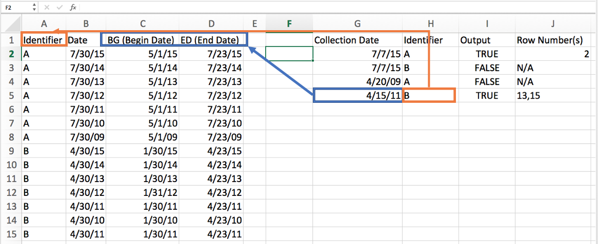
Logical functions like IF, AND, and OR are commonly used in Excel formulas to perform conditional calculations based on certain criteria. When working with date ranges, these logical functions can be extremely useful. For instance, you might want to calculate the total sales for a specific month within a given date range. In this case, you could use an IF function combined with the AND function to check if each individual sale falls within the desired month and date range.

=SUMIFS(sum_range,date_range,">="&start_date,date_range,"<="&end_date)

In this formula example, “sum_range” refers to the range of values you want to sum (e.g., sales amounts), while “date_range” represents the range of dates associated with those values. The “&” symbol is used for concatenation, allowing you to combine text strings with cell references or values. By utilizing these logical functions along with appropriate cell references, you can easily perform calculations based on specific date ranges.

Summing values within specific date ranges

Another common task when working with date ranges in Excel is summing values that fall within a particular range. This can be achieved using the SUMIFS function, which allows you to specify multiple criteria for summing values. For example, if you have a list of expenses with corresponding dates and categories, you can use the SUMIFS function to calculate the total expenses for a specific category within a given date range.

=SUMIFS(expense_amounts,expense_dates,">="&start_date,expense_dates,"<="&end_date,expense_categories,"Category")

In this formula example, “expense_amounts” refers to the range of expense amounts, “expense_dates” represents the range of dates associated with those expenses, and “expense_categories” specifies the range of categories. By setting appropriate criteria using cell references or values combined with logical operators such as “>=” and “<=”, you can easily sum values that meet your desired date range conditions.

Examples of using date ranges in lookup and conditional formatting formulas

Date ranges can also be incorporated into lookup functions like VLOOKUP or HLOOKUP to retrieve information based on specified criteria. For instance, suppose you have a table containing sales data for different products across various dates.

Mastering Excel Formulas Date Range

We started by understanding different date formats in Excel and then learned how to input start and end dates efficiently. Next, we delved into creating dynamic date ranges, calculating date differences, and manipulating week numbers and weekdays. Finally, we discussed the application of date ranges in Excel formulas.

Now that you have a solid foundation in Excel formulas for date ranges, it’s time to put your knowledge into practice. Experiment with different formulas and functions mentioned throughout the sections to gain confidence in working with dates effectively. Remember to pay attention to the details when dealing with complex calculations involving dates.

FAQs

How can I calculate the number of days between two specific dates?

To calculate the number of days between two specific dates in Excel, subtract the earlier date from the later date using the formula =later_date - earlier_date. The result will be displayed as the number of days.

Can I use conditional formatting based on a date range?

Yes, you can use conditional formatting based on a date range in Excel. Select the cells you want to format, go to “Home” tab > “Conditional Formatting” > “New Rule.” Choose “Use a formula to determine which cells to format,” enter your desired formula based on the given conditions, and specify your formatting style.

How do I extract only the month or year from a given date?

To extract only the month from a given date in Excel, use =MONTH(date). Similarly, for extracting only the year from a given date, use =YEAR(date).

Is there an easy way to add or subtract months from a given date?

Yes! You can add or subtract months from a given date using the EDATE function in Excel. For example, to add 3 months to a date in cell A1, you can use the formula =EDATE(A1, 3).

Can I calculate the average of values within a specific date range?

Certainly! To calculate the average of values within a specific date range, you can use the AVERAGEIFS function in Excel. Specify your desired criteria for both dates and values, and Excel will provide you with the average based on those conditions.